[PGP-I FM] St. Petersburg Paradox and Expected Utility

You may read in detail about the St. Petersburg Paradox and its history here, but here is the problem Nicolaus Bernoulli posed, which Daniel Bernoulli set out to solve in his book:

St. Petersburg Paradox

Consider a gamble that involves the coin-toss game. You toss a coin, and if you get ‘heads’ ( $H$ ), you get $2$ bucks and the game ends. If you get ‘tails’ ( $T$ ), however, you keep on playing till you get an $H$ at which point the game ends. Your payoff if $H$ turns up after $n$ coin tosses is $2^n$ . Nicolaus Bernoulli asked the following question – how much should you pay to play this game?

The first step towards answering this question is to ask what do I expect to win from this gamble?

Because the probability of winning $2$ bucks is $1/2$ (the probability of $H$ in the first coin toss is $\displaystyle 1/2$ ), and that of winning $4$ bucks is $\displaystyle 1/4$ (the probability that first toss turns up a $T$ , and the next one $H$ is $1/4$ ), and, in general, that of winning $2^n$ bucks is $1/2^n$ .

The expected value, then, of the winnings, say $X$ , from this gamble is:

$\displaystyle \begin{aligned} E[X] &= \frac{1}{2} 2 + \frac{1}{4} 2^2 + \frac{1}{8} 2^3 + ... + \frac{1}{2^n} 2^n + ... \\& = 1 + 1 + 1 + 1 + ... \\& \to \infty \end{aligned}$

That is, if one were to rely only on math, the answer would be a very large number. As long as there is a finite chance of $H$ turning up after a very very long time ( $n \to \infty$ ) – that is there is a positive probability of winning $2^n$ – math tells us that the expected value is infinity.

However, if you were to ask this to real people, as we did, it turns out this isn’t quite the case. In fact, when Daniel Bernoulli asked his friends this question no one seemed to be willing to pay more than a few ducats. So what is going on here? People aren’t willing to pay even a fraction of what the bet promises, but the expected value, $E[X] \to \infty$ . This is the St. Petersburg Paradox.

Daniel Bernoulli resolved this paradox by saying, and I quote:

The determination of the value of an item must not be based on the price, but rather on the utility it yields…. There is no doubt that a gain of one thousand ducats is more significant to the pauper than to a rich man though both gain the same amount.

As far back as then Daniel understood our familiar concave utility functions. And thus he argued that we should not be looking at the payoffs per se but what they offer us – that is their utility. So the quantity to be considered should be not $E[X]$ , but $E[U(X)]$ . That is, he said we should look at:

$\displaystyle E[U(X)]= \frac{1}{2} U(2) + \frac{1}{4} U(2^2) + \frac{1}{8} U(2^3) + ... + \frac{1}{2^n} U(2^n) + ...$

So far so good. But we can’t do much with a quantity written in terms of utility functions. It’s hard to quantify what is the expected utility if we just leave it like that. More importantly, it doesn’t still provide the answer to the original question – how much one should pay to play this gamble?

Daniel answered this problem by giving a functional form to the utility curve. He understood that it should be concave, and he obviously also understood its familiar properties – i.e. a pauper values a little bit of money more than a rich man (diminishing marginal utility).

He posited that a reasonable functional form for a well behaved concave utility function is 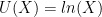$U(X) = ln(X)$ : i.e. the utility of the consumption amount $X$ is natural logarithm of the consumption amount, i.e. $ln(X)$ . You may check that it satisfies the properties for a reasonable utility curve (again, diminishing marginal utility).

And what do we get when we put $ln(X)$ in our expected utility equation:

$\displaystyle \begin{aligned} E[U(X)] &= \frac{1}{2} U(2) + \frac{1}{4} U(2^2) + \frac{1}{8} U(2^3) + ... + \frac{1}{2^n} U(2^n) + ... \\& = \frac{1}{2} ln(2) + \frac{1}{4} ln(2^2) + \frac{1}{8} ln(2^3) + ... + \frac{1}{2^n} ln(2^n) + ... \\& = \frac{1}{2} ln(2) + \frac{1}{4} (2 ln(2)) + \frac{1}{2} (3 ln(2)) + ... + \frac{1}{2^n} (nln(2)) + ... \\ & = \big (\frac{1}{2} + \frac{2}{4} + \frac{3}{2^3} + \frac{4}{2^4} + \frac{5}{2^5} + ... \big) ln2 \\&= \big( \sum_{n=1}^{\infty} \frac{n}{2^n} \big) ln2 \end{aligned}$

where we have used the result $ln(x^n) = nln(x)$ .

The term $\displaystyle \sum_{i=1}^{\infty} \frac{n}{2^n}$ is a GP which sums to $2$ (WolframAlpha confirms). The expected utility expression then simplifies to:

$E[U(X)] = 2ln2 = ln4$

That is, if expected utility is a good measure of value of something, one would be willing to pay $4$ bucks. And it turns out to be to close to the average price that people are willing to pay to play such a gamble (assuming you are not a Bill Gates, that is). So our textbook choice of a concave utility function is perhaps not that bad a choice after all.

The take-away:

When valuing risky gambles, think in terms of Expected Utility and not Expected Payoff.

…

Suggested Readings

Daniel Bernoulli’s original ‘book’ (it’s only 15 pages and fun to read): Exposition of a New Theory on the Measurement of Risk. You can find it here.

Gregory Zuckerman, The Greatest Trade Ever: The Behind-the-Scenes Story of How John Paulson Defied Wall Street and Made Financial History. Crown Business, 2009. [John Paulson bet ‘against the market’ – i.e. took a very risky gamble (John probably would disagree) – when the sub-prime boom was at its peak. He made tons of money when the bubble finally burst!]

[PGP-I FM] St. Petersburg Paradox and Expected Utility

Published by Vineet

2 thoughts on “[PGP-I FM] St. Petersburg Paradox and Expected Utility”

Leave a comment Cancel reply

Share this:

Related

Published by Vineet

2 thoughts on “[PGP-I FM] St. Petersburg Paradox and Expected Utility”

Leave a comment Cancel reply